Calculate Limb Darkening Coefficients
To calculate the limb darkening coefficients, we need a model grid.
In our first example, we use the Phoenix ACES models but any grid can be loaded into a modelgrid.ModelGrid() object if the spectra are stored as FITS files.
Two model grids are available in the EXOCTK_DATA directory and have corresponding child classes for convenience. The Phoenix ACES models and the Kurucz ATLAS9 models can be loaded with the modelgrid.ACES() and modelgrid.ATLAS9() classes respectively.
We can also use the resolution argument to resample the model spectra. This greatly speeds up the caluclations.
from exoctk import modelgrid
model_grid = modelgrid.ACES(resolution=700)
print(model_grid.data)
1056 models loaded from $EXOCTK_DATA/modelgrid/ACES/
 Teff  logg FeH          DATE        ...    Lbol       PHXMXLEN                            filename
------ ---- ---- ------------------- ... ---------- ------------- ----------------------------------------------------------
5800.0  3.0  0.0 2013-02-13 17:35:34 ... 1.5138e+35 1.51295483542 lte05800-3.00-0.0.PHOENIX-ACES-AGSS-COND-SPECINT-2011.fits
7600.0  5.0  0.5 2013-02-16 04:47:14 ... 5.4735e+33  1.3609992311 lte07600-5.00+0.5.PHOENIX-ACES-AGSS-COND-SPECINT-2011.fits
4100.0  5.0  0.0 2013-02-13 22:12:53 ... 1.3493e+32 1.90153163552 lte04100-5.00-0.0.PHOENIX-ACES-AGSS-COND-SPECINT-2011.fits
6900.0  4.0 -0.5 2013-02-15 21:47:15 ... 3.6783e+34 1.21685706454 lte06900-4.00-0.5.PHOENIX-ACES-AGSS-COND-SPECINT-2011.fits
4400.0  3.0  0.5 2013-02-16 08:31:04 ... 2.8855e+34 1.74780474088 lte04400-3.00+0.5.PHOENIX-ACES-AGSS-COND-SPECINT-2011.fits
   ...  ...  ...                 ... ...        ...           ...                                                        ...
3300.0  3.0  0.5 2013-05-19 00:40:52 ... 5.1356e+33 2.10354852144 lte03300-3.00+0.5.PHOENIX-ACES-AGSS-COND-SPECINT-2011.fits
3500.0  4.0 -0.5 2013-05-18 22:00:26 ... 6.2657e+32 2.19676308175 lte03500-4.00-0.5.PHOENIX-ACES-AGSS-COND-SPECINT-2011.fits
3600.0  5.0  0.0 2013-05-18 20:36:44 ... 6.1832e+31 2.29007335395 lte03600-5.00-0.0.PHOENIX-ACES-AGSS-COND-SPECINT-2011.fits
5700.0  4.0  0.0 2013-02-13 18:07:17 ... 1.1689e+34 1.57574414643 lte05700-4.00-0.0.PHOENIX-ACES-AGSS-COND-SPECINT-2011.fits
6600.0  3.0 -0.5 2013-02-15 21:12:48 ... 3.2868e+35 1.09919895654 lte06600-3.00-0.5.PHOENIX-ACES-AGSS-COND-SPECINT-2011.fits
6000.0  4.0  0.5 2013-02-16 05:32:33 ... 1.5904e+34 1.53258079748 lte06000-4.00+0.5.PHOENIX-ACES-AGSS-COND-SPECINT-2011.fits
Length = 1056 rows
Now let’s customize it to our desired effective temperature, surface gravity, metallicity, and wavelength ranges by running the customize() method on our grid.
model_grid.customize(Teff_rng=(2500,2600), logg_rng=(5,5.5), FeH_rng=(-0.5,0.5))
12/1056 spectra in parameter range Teff:  (2500, 2600) , logg:  (5, 5.5) , FeH:  (-0.5, 0.5) , wavelength:  (<Quantity 0. um>, <Quantity 40. um>)
Loading flux into table...
100.00 percent complete!
Now we can caluclate the limb darkening coefficients using the limb_darkening_fit.LDC() class.
from exoctk.limb_darkening import limb_darkening_fit as lf
ld = lf.LDC(model_grid)
We just need to specify the desired effective temperature, surface gravity, metallicity, and the function(s) to fit to the limb darkening profile (including ‘uniform’, ‘linear’, ‘quadratic’, ‘square-root’, ‘logarithmic’, ‘exponential’, and ‘nonlinear’).
We can do this with for a single model on the grid:
teff, logg, FeH = 2500, 5, 0
ld.calculate(teff, logg, FeH, 'quadratic', name='on-grid', color='blue')
Closest model to [2500, 5, 0] => [2500.0, 5.0, 0.0]
Saving model 'ACES_2500.0_5.0_0.0'
Bandpass trimmed to 0.05 um - 2.5999 um
1 bins of 100 pixels each.
Or a single model off the grid, where the spectral intensity model is directly interpolated before the limb darkening coefficients are calculated. This takes a few seconds when calculating:
teff, logg, FeH = 2511, 5.22, 0.04
ld.calculate(teff, logg, FeH, 'quadratic', name='off-grid', color='red', interp=True)
Interpolating grid point [2511/5.22/0.04]...
Run time in seconds:  5.451060056686401
Saving model 'ACES_2511_5.22_0.04'
Bandpass trimmed to 0.05 um - 2.5999 um
1 bins of 100 pixels each.
Now we can see the results table using the following command:
print(ld.results)
  name    Teff  logg FeH   profile   filter ...          bandpass          color   c1    e1    c2    e2
-------- ------ ---- ---- --------- ------- ... -------------------------- ----- ----- ----- ----- -----
 on-grid 2500.0  5.0  0.0 quadratic Top Hat ... <Filter 'Top Hat' from ''>  blue 0.218 0.024 0.391 0.033
off-grid 2511.0 5.22 0.04 quadratic Top Hat ... <Filter 'Top Hat' from ''>   red 0.224 0.025 0.398 0.033
Using a Photometric Bandpass
Above we caluclated the limb darkening in a particular wavelength range set when we ran the customize() method on our core.ModelGrid() object.
Additionally, we can calculate the limb darkening through a particular photometric bandpass.
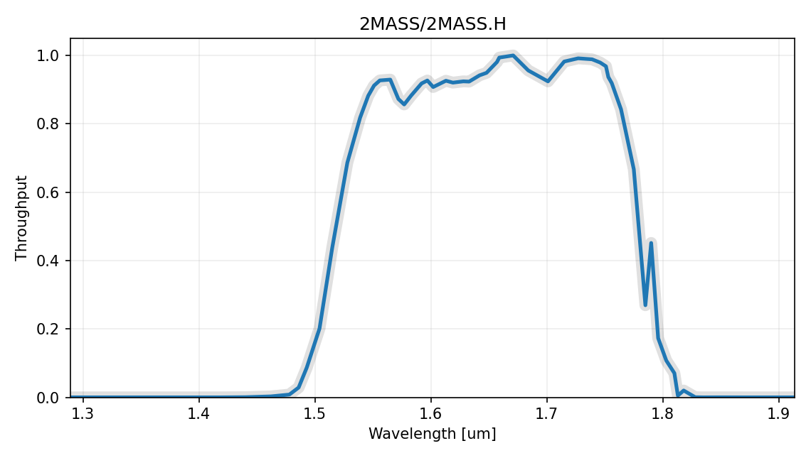
First we have to create a svo_filters.svo.Filter() object which we can then pass to the calculate method. Let’s use 2MASS H-band for this example.
from svo_filters import svo
H_band = svo.Filter('2MASS.H')
H_band.plot()
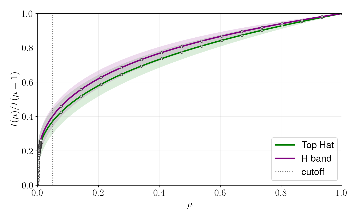
Now we can tell LDC.calculate() to apply the filter to the spectral intensity models before calculating the limb darkening coefficients using the bandpass argument. We’ll compare the results of using the bandpass (purple line) to the results where we just used the wavelength window of 1.4-1.9 \(\mathcal $mu$ m\) (green line).
ld = lf.LDC(model_grid)
teff, logg, FeH = 2511, 5.22, 0.04
ld.calculate(teff, logg, FeH, '4-parameter', name='Top Hat', color='green', interp=True)
ld.calculate(teff, logg, FeH, '4-parameter', bandpass=H_band, name='H band', color='purple', interp=True)
ld.plot(show=True)
Interpolating grid point [2511/5.22/0.04]...
Run time in seconds:  5.915054082870483
Saving model 'ACES_2511_5.22_0.04'
Bandpass trimmed to 0.05 um - 2.5999 um
1 bins of 100 pixels each.
Using a Grism
Grisms are also supported. We can use the whole grism wavelength range (as if it was a bandpass) or truncate the grism to consider arbitrary wavelength ranges by setting the wave_min and wave_max arguments.
from astropy import units
G141 = svo.Filter('WFC3_IR.G141', wave_min=1.11*units.um, wave_max=1.65*units.um, n_bins=15)
G141.plot()
Bandpass trimmed to 1.11 um - 1.65 um
15 bins of 431 pixels each.

Now we can caluclate the LDCs for each of the 15 wavelength bins of the G141 grism we just created, where the first column in the table is the bin center. This is not very useful to plot but… why not?
teff, logg, FeH = 2511, 5.22, 0.04
ld = lf.LDC(model_grid)
ld.calculate(teff, logg, FeH, '4-parameter', bandpass=G141, interp=True)
print(ld.results)
Interpolating grid point [2511/5.22/0.04]...
Run time in seconds:  5.983066082000732
Saving model 'ACES_2511_5.22_0.04'
 name  Teff  logg FeH    profile        filter      ...   c2     e2    c3     e3    c4     e4
----- ------ ---- ---- ----------- ---------------- ... ------ ----- ------ ----- ------ -----
1.125 2511.0 5.22 0.04 4-parameter HST/WFC3_IR.G141 ...  0.418 0.011 -0.599 0.011  0.193 0.004
1.155 2511.0 5.22 0.04 4-parameter HST/WFC3_IR.G141 ... -1.135 0.016  0.454 0.017 -0.071 0.006
1.186 2511.0 5.22 0.04 4-parameter HST/WFC3_IR.G141 ... -1.065  0.01  0.458 0.011 -0.086 0.004
1.218 2511.0 5.22 0.04 4-parameter HST/WFC3_IR.G141 ...   -1.3  0.01    0.7 0.011 -0.168 0.004
1.250 2511.0 5.22 0.04 4-parameter HST/WFC3_IR.G141 ... -0.838 0.008  0.321 0.009 -0.052 0.003
...    ...  ...  ...         ...              ... ...    ...   ...    ...   ...    ...   ...
1.427 2511.0 5.22 0.04 4-parameter HST/WFC3_IR.G141 ...  0.947 0.012 -0.775 0.013  0.209 0.005
1.465 2511.0 5.22 0.04 4-parameter HST/WFC3_IR.G141 ...  0.916 0.033 -0.893 0.035  0.273 0.013
1.504 2511.0 5.22 0.04 4-parameter HST/WFC3_IR.G141 ...  0.611 0.037 -0.776 0.039   0.26 0.015
1.544 2511.0 5.22 0.04 4-parameter HST/WFC3_IR.G141 ...  0.291  0.05 -0.623 0.053  0.235  0.02
1.586 2511.0 5.22 0.04 4-parameter HST/WFC3_IR.G141 ... -0.825  0.01  0.308 0.011 -0.049 0.004
1.628 2511.0 5.22 0.04 4-parameter HST/WFC3_IR.G141 ... -1.126 0.005   0.57 0.005 -0.131 0.002
Length = 15 rows
Calculating SPAM Coefficients
The 4-parameter coefficients can also be transformed into Synthetic-Photometry/Atmosphere-Model (SPAM) coefficients. SPAM coefficients depend on the planet geometry, so the calculation needs either a planet_name that can be resolved by ExoCTK or an explicit planet_data dictionary. Supplying the dictionary directly keeps the calculation reproducible and avoids a remote query.
planet_data = {
    'transit_duration': 0.10,
    'orbital_period': 3.0,
    'Rp/Rs': 0.1,
    'a/Rs': 10.0,
    'inclination': 88.0,
    'eccentricity': 0.0,
    'omega': 90.0,
}

ld.spam(planet_data=planet_data, profiles=['quadratic'], ndatapoints=200)
print(ld.spam_results[['name', 'profile', 'c1', 'c2']])
 name  profile    c1    c2
----- --------- ----- -----
1.125 quadratic 0.294 0.362
1.155 quadratic  0.22 0.314
1.186 quadratic 0.223 0.315
1.218 quadratic 0.192 0.295
1.250 quadratic 0.209 0.306
...       ...   ...   ...
1.427 quadratic  0.36 0.406
1.465 quadratic 0.336  0.39
1.504 quadratic 0.294 0.363
1.544 quadratic 0.274 0.349
1.586 quadratic 0.209 0.306
1.628 quadratic 0.182 0.288
Length = 15 rows
The full ld.spam_results table also keeps the planet properties used for the transformation, along with the original filter and model-grid metadata.